Example of a Color Negative Scan

On the left in fig. 4 is a raw scan of an ISO 100/21 transparency. On the right is the raw scan of the same scene on an ISO 100/21 negative film shot under the same lighting. Both were scanned as transparencies using the scanner's autoexposure, 500 dpi, and at 8-bits.

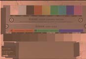
fig. 4

The grayscale control strips were extracted from the raw scans and horizontally flipped:

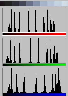
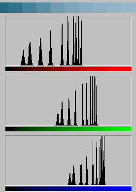
fig. 5. Left, RGB histograms for grayscale on transparency. Right, RGB histograms for grayscale on negative (inverted to match order of transparency's). Note horizontal placement of color intervals reflect the vertical displacement in the Kodacolor-100 characteristic curve, previous page, e.g. the blue curve has the greatest vertical displacement and thus has its intensity interval shifted furthest to the right. In addition, one would think that because the 3 channels can each result in a range of 2 orders of magnitude of density the distributions should be of equal widths. Histograms display intensity values (0 to 255), however, not density values to which the relationship is inversely proportional. The widths of the distributions reflect the effect of the offsets in translating density to intensity. For example, because its upwards displacement in the characteristic graph is greatest, blue spans the fewest intensity values (its domain is smallest)

Each step is readily identifiable as a cluster in the histogram. The narrow histogram ranges for the negative are typical. The wide footprint left by the orange mask is evident in the constricted blue and green tonal ranges, the complements of orange (lots of yellow plus some magenta), but blue is the critical channel because it is more severely impacted.

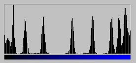
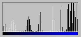
fig. 6; histograms of blue channels after black-white point setting applied. Left, transparency; right, negative

Fig. 6 shows the histograms after the black and white points have been set for the two grayscales. For the color negative scan the range of values encompassed by the blue component for each step has been smeared over a wider range of values by spreading the bars. The step clusters in the transparency are affected little because the range undergoes minimal expansion.

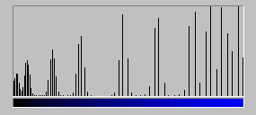
fig. 7; histogram of blue channel from the negative after gamma correction to match printed and transparency tones

We still haven't finished adjusting the negative scan image: after the black and white points are set, a fairly strong gamma correction curve to darken (fig. 7) must be applied to match the tonalities seen on the print and transparency versions. (Note the approximate positional correspondence of the clusters to the transparency's [left, fig. 6]. The necessity of applying the gamma correction seems to be common to all [C-41] negative color films that I've tried, not particularly to this example.) After applying the curve, some of the step clusters have suffered so much from the manipulations that they are no longer individually identifiable. In the shadows some of the steps have begun to merge; in the mid- and high-light tones enlarged gaps within the steps are obvious.

4x, 14-bits

16x, 14-bits

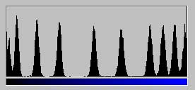
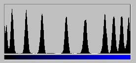
fig. 8

Fig. 8 shows the final blue channel histograms for the same negative scanned at 14-bits and 4x and 16x multi-sampling. Variations in intensity in the steps (indicated by the spread bases of the clusters) are about equal in size and are caused by imperfections in the film image: differences in lighting, grain, etc. Any differences caused by scanner inaccuracy are too small in comparison to have an effect on the histograms.

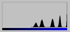fig. 9

The negative in fig. 4 was also scanned on an inexpensive flatbed with a transparency adapter. Fig. 9, from the raw scan, shows that the scanner was unable to resolve the 6 darkest blue steps. Compare this to the negative blue channel in fig. 5.