|
Contents Understanding Image Histograms and Curves Histograms Histograms and Pixel Structure Using Histograms as a Scanner Tool Image Exposure and Tone Curves Changing Brightness and Contrast Interactive Demos Appendices The Photoshop Levels Function and Curves |
Another important diagnostic tool is what I call the local histogram, as contrasted to the global histogram, which summarizes the entire image. A local histogram samples an area of particular interest lying within the image, a spatial subset.
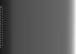
Returning to our tonal gradient, we'll construct a rectangular selection (dotted line), which defines the area to be measured by the histogram function:
 |
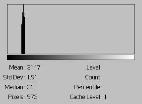 |
fig. 9
The histogram shows that the values are within an extremely narrow range of values. In contrast to the global histogram, this local histogram tells us we are examining a nearly solid tone. Even without seeing the selection, one could guess the shape, location, and size of the selection.
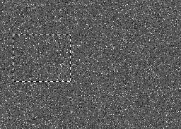
Returning to our second image (fig. 7), where we've taken the first image and randomly moved the pixels, we'll make another rectangular selection:
 |
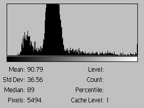 |
fig. 10
This local histogram is almost exactly the same as the global histogram. This makes sense because the pixels are arranged randomly, so a large enough sample is representative of the distribution of pixels of the entire image. In this image there is no privileged view. A privileged view is a local view that offers information about where it is in the global view. For this image, any view should have the same histogram as the global as well as any other local view.
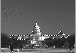
For the third picture (fig. 8), instead of a rectangular selection, we'll draw the selection around the US Capitol Building, the subject of the picture.
 |
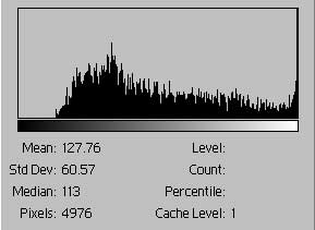 |
fig. 11
This histogram shows a fairly well distributed range of tonal values from the mid-tones to the highlight tones. Some of the pixels have gone to complete white. This is not unexpected since the capitol is made of white limestone. The global histogram is darker, the mean value is 91, and has a much lower standard deviation of tone. A change in contrast will have a greater effect on the subject area than the rest of the image.
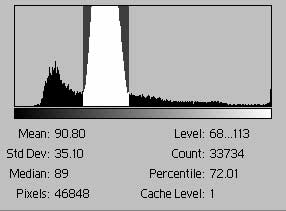
Much of the area of the image (about 72%) is of the sky. Only a few hundred or so of the subject's pixels are in this hump (white area).
There is a feedback mechanism between local histograms and the global histogram. In general, the local histogram will be associated with the area of the image containing the subject. When it comes to adjusting the image, as you make changes to one, global or local, you'll want to check the effect changes have on the other.
Image Detail Size Affects Apparent Contrast
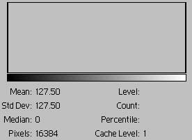
It's obvious that fig. 12 is maximally contrasty (the standard deviation is 127.5). Locally, on the pixel level, however, it would have zero contrast. Fig. 13 appears to be a monochromatic gray with no contrast at all. Yet it is composed of alternating black and white pixels, exactly the same pixel elements as fig. 12 but arranged differently. Therefore, according to the histogram, it also has maximum contrast. Note that fig. 13 has only bars at the extremes. Locally, on the pixel level and in contrast to fig. 12, it would have maximum contrast. So 12 and 13 differ in their local contrast. Of course, this is a most extreme case, but pointillistic effects often lead to subjective judgments counter to the histogram's purely objective display. Why is this detail important? Curves might have radically different effects depending on local contrast. If fig. 13 were instead mid-tone gray pixels, it would behave differently in response to a tone curve.

fig. 12 |
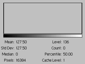 |
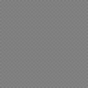
fig. 13 |
 |
(The half-tone gray in fig. 13, can be converted into a real gray by using the contrast slide control. Decreasing contrast will shift the black and white pixels towards each other in tone.)
A local histogram used with the image histogram enables the scanner operator to vary the allocation of the available tonal range between the subject and the image as a whole
![]()
![]()