Postscan Histograms

Histograms displayed by scanner programs are formed by sampling the image preview. A histogram of the final image, obtainable in an image processing program such as Photoshop, gives a more accurate representation of the image's characteristics. It is useful when it is necessary to examine the histogram in detail.

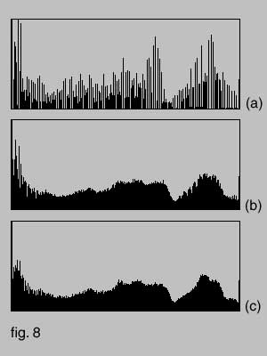Note the vertical bar at the left margin, implying a high number of tones that could not be imaged. In addition, the relatively smooth contours of distributions 8b and 8c degenerate near the left tails. This is because this area is near the limits of the scanner's density range, where pixel values are more likely to be distorted by noise and thus exhibit greater randomness. This does not necessarily mean that the scan will be unacceptable. It does demonstrate the effectiveness of the histogram in indicating potential problems.

Fig. 8 shows a progression in image quality for 3 scans of the same image. Fig. 8a is for an image which has been tonally adjusted by using curves. Note the development of drop-outs. Some tones have combined with adjacent tones to form tall spikes and leave gaps indicating their absence. Fig. 8b is for the same image, but tonal adjustment has been achieved by using analog gain rather than curves. Fig. 8c is the same as 8b but in addition was scanned in 12-bit mode. As a result it exhibits the smoothest contour of the three scans, although in practice 8b and 8c would be visually identical in appearance. Both 8b and 8c efficiently use the tonal space since all values are used.

fig. 9a

Using Multi-Sampling

The effectiveness of multi-sampling to suppress noise relies on the premise that errors in reading pixel values are non-systematic, i.e. truly random. Thus they can be eliminated by scanning the image several times and taking an average value for each pixel. Implementing this in software requires making several copies of the image as a source for the final image. Some scanners do this in hardware by taking up to 16 readings at each position as the CCD sensor array is stepped over the image. This has the advantage of maintaining registration and performing the task in one pass.

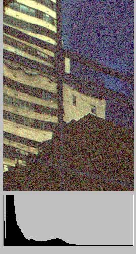
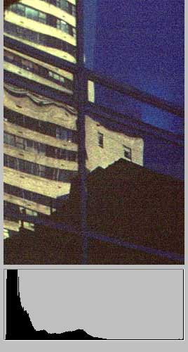
Fig. 9 shows the effect of using of multi-sampling in reducing noise near the limits of the scanner's sensitivity. The scan for the histogram for 9a was performed without multi-sampling and shows an erratic contour at its left edge, showing the effects of noise. Fig. 9b, performed with 16x sampling, has a clearly defined contour at its left edge. (Details shown above histograms.)

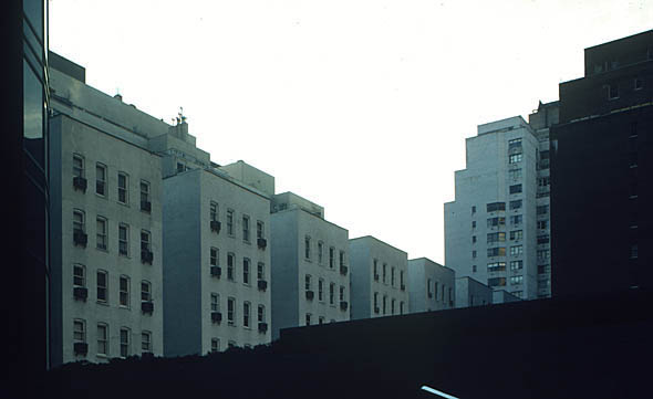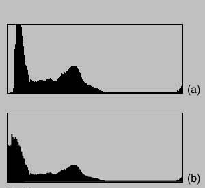
fig. 10

Fig. 10a, the histogram for the picture above, has three salient features. The dark foreground appears as the largest peak on the left. The buildings are represented as the mid-tone peak. An essentially featureless sky in the source transparency was forced into white (the peak along the right margin) so that the building features and foreground tones could occupy more of the tonal space. It is important to emphasize that the foreground is not black and contains detail.

Fig. 10b is a hypothetical histogram for the same image scanned on a scanner with a more limited density range. Because many of the picture's tones are beyond the scanner's ability to image them they become black (black line against left margin).

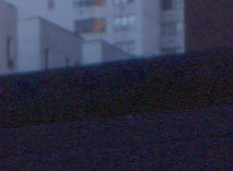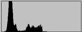fig. 11

In reality, the typical behavior for scanners with a limited density range is shown in the detail in fig. 11. Non-imageable areas become noise, which register as non-black tones instead. Figs. 10 and 11 emphasize the importance of the area near the black end-point in a scanner histogram.

A Histogram for Negative Film is the Reverse of a Histogram for Transparency Film

The examples I have used so far have been from transparencies. For negative film, of course, the reverse applies--it is the area near the right end, the highlight end-point, that is more important. This is where the pixel values for the densest areas on film will appear. Fortunately for amateur photographers, negative film tends to be more scanner friendly than transparency film because the densest tones are not as dense as the densest tones on transparency film, thus avoiding the limitations of the scanner's density range. Kodachrome, a transparency film, with its nearly opaque dark areas, for example, can be particularly challenging for most scanners. To say it is the bête noire of scanners seems particularly apt. For the sake of simplicity, this tutorial assumes the use of transparency film.

Look for Bars of Maximum Height along Either Margin

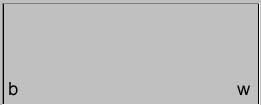A bar of maximum height at either margin (b, w) may signal a loss of tonal separation.

The cause may be a tone curve that has thrown values into the extremes; tones beyond the capability of the scanner to image; or truly characteristic of an unusual image.

Indicators of a loss of tonal separation -- merged bars, such as fig. 8a, bars along the margins, discontinuities, or rough contours in larger images -- imply a loss of information in the image.

In preparing an image for production, some loss of information is inevitable, even desirable if the image's main elements are to be emphasized. The importance is in knowing how to control information loss as a means of enhancing the production image.