Image Histograms

How does one judge a scanned picture? More basically, what are the criteria by which one judges the quality of a scan? Conceptually simple factors such as focus and frame alignment are immediately obvious from viewing the monitor and are easily adjustable through simple controls or manual adjustment. Other factors such as color and tonal balance are much more difficult to evaluate by looking at the scanned image on the monitor. A full-frame scan on a scanner with a default resolution of 1350 dots per inch will generate approximately 6 million bytes. At a resolution of 2700 dpi, the file will contain over 24 million bytes. Obviously no one is intellectually capable of following such a mass of points individually. At the other extreme, the person who can consistently obtain quality scans by just previewing images on the monitor is exceptionally talented indeed.

An image histogram is a way of making quantitative sense of this mass of data.

A brief course on histograms

One of the characteristics of an image that we want to analyze is the lightness or darkness of its pixels, or luminosity. An image of tone steps is a good introduction to understanding image histograms because similar tones are grouped together, making the correspondence between pixel count of each tone (the area of each tone) and bar height obvious:

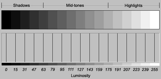
fig. 1a

Luminosity values range from 0 (black) to 255 (white) and are whole positive numbers; there can be no 22.5, -10.0, 156.19, etc. In fig. 1a each of the 17 steps contains 2048 pixels, so the height of each bar underneath represents a count of 2048. This histogram has a fixed-height vertical axis, which is set equal to the tone with the greatest frequency (the statistical mode). The heights of the other bars are then set relative to the tone with the greatest frequency. Since the steps in this example are equal in size -- have the same number of pixels -- the bars are equal in height.

In this image, the fifth step is doubled in size to demonstrate that histogram bar heights are relative to the sample with the greatest frequency and are not absolute:

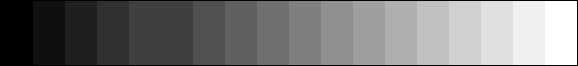
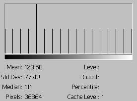fig. 1b

Here's something much simpler:

Single tone, no contrast

fig. 2

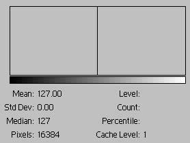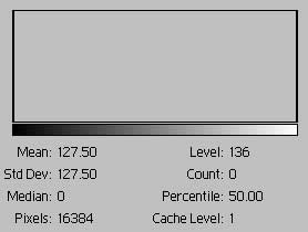
This is as simple as it gets, a one color-one bar histogram. The RGB levels of the color are (127, 127, 127). The bar has a height of 16,384 -- all the pixels in the image. As a result the mean and median are 127. The bar's height could also be read as 100%, a percent scale, since that's the only color. With every pixel having the same tone, the standard deviation is zero.

Two tones, high contrast

fig. 3a

This image is 50% black and 50% white. The bar at the extreme left represents the frequency of black and has a height of 8192; the bar at the extreme right represents the frequency of white and has a height of 8192. The average tone is the same as in fig. 1a, but a gray tone of this value is not present in the image. The extreme difference in tones is indicated in the high standard deviation -- a pixel is either black or white. The standard deviation is useful as a numerical proxy for the contrast of the entire image. The median is incorrect and should be 127.5.

Two tones, high contrast

fig. 3b

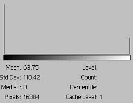In fig. 3b we've changed the proportions of black to white pixels to 3 to 1. That is 12,288 pixels are black and 4096 are white. As a result, the black bar is 3 times higher than the white bar. The histogram frame has been removed to make this clearer.

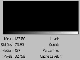fig. 4

Fig. 4 is a scale of 256 gray tones that appears continuous. The histogram is solid with bars because the continuous gradation has no missing tones.

An image histogram consists of 1 to 256 tonal values, or bars

The height of each bar represents the count of pixels having that tonal value (0 to 255)