|
Contents Understanding Image Histograms and Curves Histograms Histograms and Pixel Structure Using Histograms as a Scanner Tool Image Exposure and Tone Curves Changing Brightness and Contrast Interactive Demos Appendices The Photoshop Levels Function and Curves |
It's a Matter of Correct Exposure
If you're serious about photography you take great care in setting your camera's exposure. A scanner is also a camera, and a possible weak link in your production chain unless similar care is taken in setting its exposure. As an exposure meter is used to monitor a camera's exposure, the histogram is the primary tool used to monitor a scanner's exposure. That's why histograms are important.
Histograms are used in scanning to show how the values of the pixels that have been captured are distributed over the scanner's tonal sensitivity range, just as a camera's meter indicates how well the image matches the film's tonal range. In other words, they tell you how efficiently the scanner is being used. Without them it would be extremely difficult to achieve technically optimal scans.
| Histograms provide a graphical display of the state of the image, summarizing the vast quantity of data contained in a typical scan | |
| It is nearly impossible to make the final adjustments through visual feedback alone. Monitors are incapable of displaying the subtle differences in the shadow areas which are easily discerned in a histogram |
These principles also apply to digital cameras which display histograms.
 |
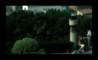 |
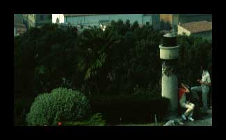
These two images illustrate the limitations of the monitor as a scan diagnostic tool. The picture on the right has more shadow detail than the one on the left. To view these differences, however, one must increase monitor brightness and contrast to the maximum -- hardly a convenient way of comparing image quality. Why should one worry about detail not visible on the monitor? For a Web application, for example, you may not need such detail, but in another application you may need that detail if some manipulation of the tones or colors make these tonal areas more visible. Or some other output medium that you may want to use, presently or in the future, may be capable of displaying these distinctions.
How the Scanning Process Relates to Image Histograms
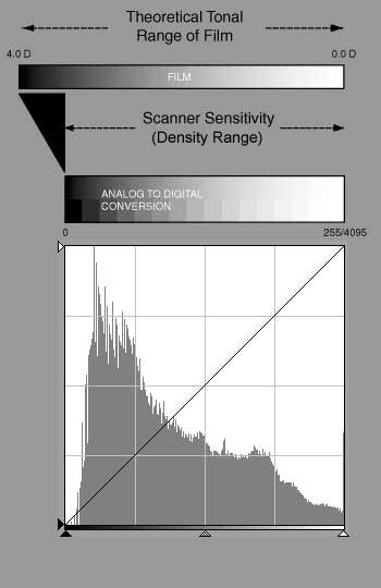
fig. 1 |
The typical scanner has a density range less than that attainable on film. Any tones denser than that perceivable by the scanner become black, also known as clipping. The width of the scanner histogram's horizontal axis--from the left (black) to right margin (white)--represents the scanner's density range. Each of the bars, of course, represents the pixel count for the tone value of its position. This particular histogram shows that approximately two-thirds of the scanned image's pixels--the dark gray area--are in the darker half of possible tonal values. The Photoshop version of the histogram for the image is functionally similar:
The scanner histogram, at left, is for the preview image, which is based on a small sample of pixels. The Photoshop histogram is for the scanned image. |
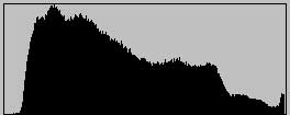
Image Density Range and Scanner Density Range
One of the primary reasons for performing a preview scan is to obtain an image histogram. Yet I would guess that because of simple ignorance the vast majority of non-professional scanner users simply ignore this extremely useful device. I would also guess the same applies to users of graphics editing programs such as Photoshop. This section gives an idea of how to begin to use histograms in scanning.
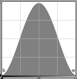
If you get fig. 2 as an initial preview histogram, this is about as good as it gets. The image's tonal range neatly matches the scanner's density range without having to apply curves adjustments. The left of the histogram (b) abuts the base of the scanner's density range and the right of the histogram (w) abuts the high-end of the range. The scanner's sensitivity is used at maximum efficiency: none of the image is outside the scanner's sensitivity range and samples will be obtained for all 256 tonal values.
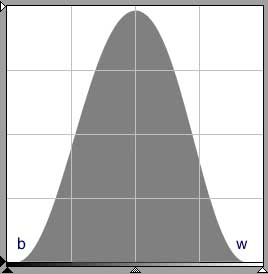 fig. 3
Fig. 3 is a histogram where both b and w are in the left-most and right-most quarters of the histogram but not touching the edges. The scanner's sensitivity is used efficiently.
Examples: Average density range, average contrast
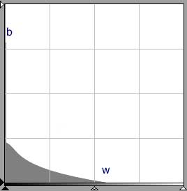 fig. 4a fig. 4a |
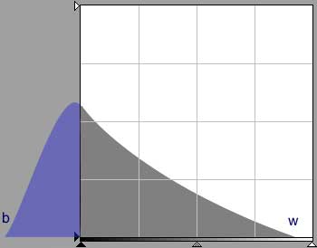 fig. 4b fig. 4b |
Fig. 4a is a histogram, most commonly encountered in scanning transparencies, where some of the film's tones are beyond the scanner's sensitivity. Fig. 4b, a notional histogram implied by fig. 4a, depicts the part of histogram (blue) falling outside the scanner's density range. The tones in the blue area are imaged as black.
Example: Wide density range, average contrast
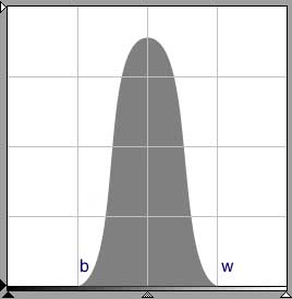 fig. 5
Fig. 5 is a histogram with endpoints close or near the quarter tone markers. This is an uncommon occurrence. Much of the scanner's density range is unused.
Example: Narrow density range, very low contrast
Evaluating the Preview Histogram
 fig. 6
 |
 fig. 7
 |
Figs. 6 and 7 are histograms for scans of the same image without curve adjustment and illustrate making use of the available density range. Even if the scan represented in fig. 6 had resulted in an image visually closer to the desired final image, the image represented by fig. 7 is preferred because it spans the range of available tone values and as a result contains more information than 6. With more information, the user has greater latitude for subsequent manipulations of the image. One could produce the image in 6 from 7 but not the reverse. Note that although figs. 6 and 7 are for the same image, fig. 7 occupies a greater area.
![]()
![]()