A Brief Note on Scanning Color Negative Film -- A Conceptual Framework

With narrow density ranges -- easily within the capabilities of most consumer scanners -- it may seem almost fortuitous that color negative films are scanner “friendly”.  On the other hand, it may seem somewhat bizarre to consider that scanning color negative film on a high-end scanner can result in unacceptable results unless one makes provision for its unique characteristics.  Whereas transparencies are more demanding of the minimum and maximum densities of scanners – and we can therefore take the approach of concentrating on exposure, color negatives are more demanding of scanner accuracy.

Considered as scanning media, other than being obvious reversals of each other, color negative and transparency film differ in that

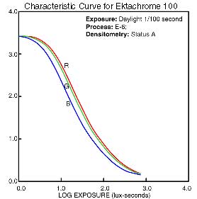
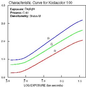
One of the advantages of transparency film is that the response curves are nearly coincident (and they'd better be!).  Consequently, achieving color balance is usually straightforward.  The response curves for color negative film, on the other hand, are at considerable offsets from each other.  The user must force them into alignment by setting the black-white points for each of the 3 channels (few people, not surprisingly, are aware that this is what they're doing in setting the black-white points).  Getting the black-white points right for color negative film is much, much more critical than transparency film.  Small errors in locating the black-white points may result in significant misalignment of the curves -- the black-white setting functions have steep slopes.  Consequently, color balance may be nearly impossible to achieve.

As a consequence of its design characteristics, a scan of color negative film results in a narrow range of density values as in fig. 1.

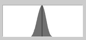
fig. 1, histogram for color negative.  Dark band indicates zone of uncertainty for a hypothetical mid-tone.  A quantized pixel value could be anywhere in the interval

Ideally, we’d like something more like this:

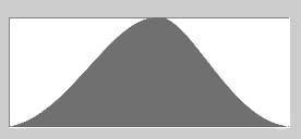  fig. 2

where the full range of intensities are represented.

But when the image for fig. 1 is expanded to set the black and white points we get:

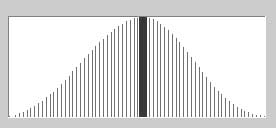
fig. 3, histogram in fig. 1 after B-W points set.  Zone of uncertainty is expanded along with intensity range.  Subsequent curve or level adjustment may magnify the error

The histogram indicates that the black and white point set image has substantial numbers of missing values (gaps).  In addition, negatives have greater latitude than transparencies so the narrow range in fig.1 potentially encodes a longer dynamic range, thus causing the gaps to be more noticeable.  Without preventative measures, scans of color negatives are more prone to posterization.

Setting the black-white points is intrinsically a contrast increasing operation (an "S" shaped curve is applied).  Negatives require more extreme contrast increases to expand their narrower density ranges, thus making more noticeable any scanner defects such as a tendency to "band".

Don’t Confuse Scanner Precision with Accuracy

Well, you may figure, my scanner can also output at 12-bits, 8 plus 4 extra bits, therefore I can have 16 (2⁴) additional values available between each of the 256 values available in 8-bit scanning.  (Think of the extra bits as values to the right of the binary point.)  So I can get those in-between gradations of gray to fill-in the potential gaps after I set the black and white points (fig. 2).  It almost seems like a free lunch.  Here’s the catch: what the scanner manufacturer didn’t tell you is how accurately your scanner is measuring those values.  So although your scanner may be sending 12-bits per color some of the 12-bits are not reliable.

By scanner accuracy, I mean that the CCD sensors can see pixels of the same intensity of light and yield consistent readings.  Suppose you have a slide with a perfect monochrome density, without blemishes, neither grain nor scratches, whatever.  Suppose it is scanned on both a low- and high-end scanner.  When the images are analyzed let’s say the resultant pixels have the same average value, 128.  If you look at the individual pixels, however, you’ll find that the values frequently vary from 128, some may be 127 or 129, etc.  The key statistic to scanner accuracy is the standard deviation.  The low-end scanner will have a high standard deviation, usually greater than 2, and the high-end scanner will have a low standard deviation, usually less than 1.  For the low-end scanner this means that even for 8-bit scans, only about 6 of those bits are reliable.  It only gets worse because when the color negative’s ranges are expanded by setting the black and white points the number of accurate bits is similarly reduced.  Admittedly, my opportunity to measure various scanners has been limited, but several high-end scanners that I’ve tried output only 8 accurate bits using single pass scanning.  Thus any bits beyond 8 essentially would avail you nothing since they’re garbage.  

Ordinarily these garbage bits could be ignored, but the narrow intensity ranges typical of color negative scans, e.g. fig. 1, require curve functions with high slope values to set the black and white points.  A curve with a high slope applied to a pixel scanned with low accuracy shifts the garbage bits into significance, causing the pixel to appear prominently as noise in the image.  For example, the dark gray band in fig. 1 indicates the possible range of error for a single mid-tone value, i.e. the resultant reading of this single intensity could fall anywhere within the range.  Setting the black and white points also expands the range of error (fig. 3).  In addition, subsequent curve and level adjustments applied to the image similarly magnify the effect of any error. This becomes most evident in image areas, such as highly saturated blue sky, containing otherwise smooth gradations in tone.  The yellow layer (blue channel) in negative color films tends to be the most constricted, suffers the greatest expansion, and therefore is the most prone to posterization.

All of this gives me the convenient opportunity to state my real grievance with color negative film.  Despite my earnest attempts at careful handling, it seems that their (thinner?) emulsions are more delicate than those on transparency films, resulting in more scratches.  These physical flaws are nicely aggravated by the exaggerated contrast enhancement required to process color negative scans.

Three Approaches to Scanning Negatives

There are three strategies to address the problem of narrow density range:

Do nothing special  If the images are family snapshots or meant for Web display, for example, taking remedial measures probably aren’t worth the time or effort since they’re unlikely to result in any visible improvement. 

Increase exposure  The problem with this is that there are huge gaps to be made-up on the left and right sides of the histogram distribution (fig. 1).  A modest increase in exposure can be made to address the gap in the highlights, but beyond that there is a cost of increased flare and noise.  At best, increasing exposure is only a partial solution.  In fact, what NikonScan, for example, seems to do is decrease exposure in its negative mode scan as compared to transparency mode.

Perform an 8+ bit scan  This is the conventional approach for critical images on color negatives.  The most obvious cost is that the image file is doubled in size to accommodate the extra bits beyond 8.  Then there is also the subtle factor of scanner accuracy, of which few scanner users, through no fault of their own, seem to appreciate.  Not taking this into account can diminish the worth of their 8+ bit scans.

For Critical Scans of Color Negatives Use Multi-Sample Mode

Multi-sample scanning partly addresses this by averaging out the errors.  Each step up will yield approximately one more extra accurate bit.  For example, 16x scans yield approximately 11 accurate bits, in this case justifying 8+ bit scanning.  The narrower the density range, the more significant bits you'll need.  So if you're going to add extra bits to your scan, it makes sense to add meaningful ones.

In summary, to achieve a full range of tones from color negatives accurately, we’ve had to double image file size and greatly increase scan time, something that belies the seeming ease of scanning them.  Having said all this for understanding (and certainly not for intimidation!), I personally have rarely, practically speaking, found it necessary to resort to such measures (but then to be honest I also rarely shoot with negative film).  Note that the histograms tend to over-dramatize the differences and it's unlikely that they'll be visible, especially in areas of the image composed of pixels of heterogeneous color.  Fortunately, the reader can easily determine for himself whether 8+ bit scanning and multi-sampling are necessary for a particular application.  What's important is knowing the issues and subsequent trade-offs.