Alternative 3 -- Scan Using Photoshop and NikonScan with Analog Gain
This is an especially effective method with films, such as Kodachrome, which are very contrasty and have extremely dense blacks. The advantage of this method is that it produces the best quality scans of slides because cranking up the luminance of the LEDs pushes more light through dark areas. The disadvantages are that it's extremely tedious -- changes in analog gain are not dynamically reflected in the preview so a new preview must be run for each change; and overdoing the master analog gain can cause detail in highlight areas to wash-out, primarily due to increased flare. Technically speaking, the rationale for this method is that the curve transformation functions map small finite integer domains (created by the scanner's ADC) into similarly small integer ranges (the image file). If you can adjust the analog readings so that the curve transformations do not need to be performed or are minimized, the inevitable loss of precision through integer computation is avoided. This method can also be combined with the approach used in "Alternative 2", where the corrections are made in Photoshop and passed back to NikonScan.
Interactive demo on adjusting exposure on the LS-2000 (with Java enabled browser)
Information flow schematic for the LS-2000
Step 2. Adjusting Tone by Adjusting Analog Gain
Prior to correcting any color casts, I first try to get a scan with acceptable tone. This is similar to the procedure that one follows in darkroom printing. This method sets the black and white points by increasing the analog gain until the histogram spans the graph. The usual practice in making a scan is to move the black and white pointers (below the horizontal axis) to meet the ends of the histogram. Here we're doing the reverse, expanding the graph to fit within the pointers.
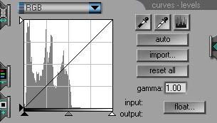 |
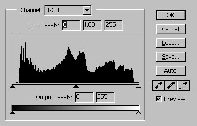
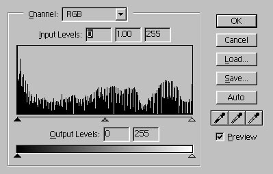
Comment: This is the preview image's histogram generated in Step 1. Normally I modify the analog gain only if the histogram occupies less than 75% of the X-axis. |
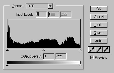
Setting master analog gain to 1.0 and re-running preview results in the histogram:
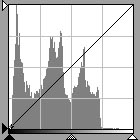 |
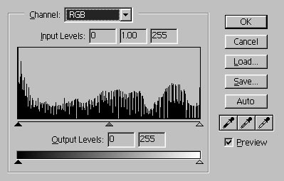
Comment: As the analog gain is increased, the right edge of the histogram will creep towards the white point. The advantage of increasing the analog gain ends when the left edge of the histogram starts drifting right at the same rate or faster. This would mean we're no longer gaining contrast. Stop increasing the analog gain. If you want to adjust the white point, you'll have to move the white pointer or modify the RGB curve. The other key indicator to be monitored during this process is flare. This is indicated if detail starts to wash out or if dark areas become muddy. Example 2 of Flare Note especially the absence of flare in the silhouetted tower in the drum scanned image as compared to the CCD scanner image. |
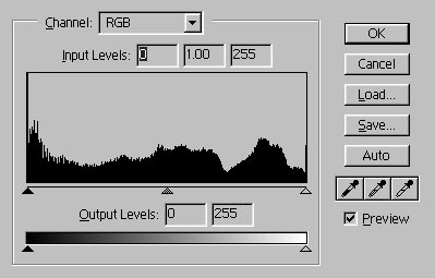
The right edge of the histogram is about half-way to the right edge (the white point). Setting master analog gain to 1.8 and re-running preview results in the histogram:
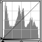 |
Comment: The range of settings for the gain of the master channel is -2.0 to 2.0. By setting the gains for the individual colors, which are added to the master channel, it is possible to go beyond this range. |
Effectively what we've done with this trick is to increase image contrast (i.e. increasing the distance between the left and right edges, c.f. tutorial) in the analog (continuous number) domain and have lost no information; we avoided increasing contrast in the discrete domain and possibly losing information. Change in contrast from scan to scan may be monitored quantitatively by making an interim image, loading it into Photoshop, and displaying the histogram, which also displays standard deviation. If it is increasing, contrast is increasing also.
This sets the RGB black and white points. Make a scan from the image to pass to Photoshop.
Step 3. Correcting the Blue Cast
Open this initial image file in Photoshop:
On the menu click Image, Adjust, Levels to display the histogram:
 |
Comment: This is the image's histogram generated in Step 2, not adjusted for blue. |
Clicking auto sets the black- and white-points for the 3 color channels.
Now the point of the exercise: correcting Kodachrome's blue cast. Basically, this cannot be accomplished by using linear correction (e.g. the sliders).
Select the blue channel
Adjust the blue channel by either moving mid-tone input level marker or editing the mid-tone number. For this picture this was at about .75.
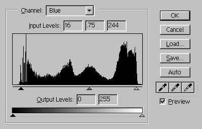
After the blue channel is set the corrected image looks like this:
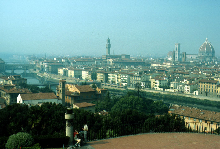
If high quality is not a concern, this can be the image used.
 |
Comment: On the other hand, note the discontinuities caused by the curves manipulations in the histogram of the image. In general, global manipulations should be performed in the scanner before the image is digitized. |
Save levels settings.
Step 4. Getting the final scan
Open the curves-level drawer in NikonScan and import the settings saved in Photoshop. Run the final scan.
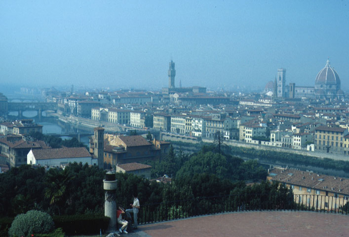
This final scan has noticeably greater shadow detail than the other alternatives (you may have to turn-up your monitor's brightness; note the trees in lower-left).

This is the Photoshop histogram of the final scan.
 |
Comment: Of the 3 methods, this method results in the smoothest histogram because tonal balance was achieved by increasing the brightness of the LEDs until the width of the histogram exactly matched the width of the X-axis rather than by using curves. |
 |
Comment: Another scan was done in 12-bits. The histogram for the 12-bit version shows a smoother histogram function, although this difference is not visible in the image (not shown). 12-bits means that there are 4096 tonal levels (rather than the 256 possible with 8-bits), enabling a finer resolution of the levels and hence a smoother curve. |
There is another variant of this method, theoretically capable of yet better results. Instead of optimizing by adjusting the analog gain for the tone, the analog gains for underlying RGB colors are adjusted individually. This is left as an exercise.
| Back to the '70s -- Fixing the Green Cast
About 1974 Kodak replaced Kodachrome II and X with Kodachrome 25 and 64. Many of the first rolls sold had a ghastly green cast, supposedly caused by insufficient aging. If you still have any of these shots, you can correct this green cast by a -0.28 (this will vary) analog gain setting for the green channel. |