Setting the Black and White Points
An essential function of preparing an image for display is that you literally
have to tell the computer what is black and what is white. Often after a
preview scan is performed, you will note a tone that should be black is lighter
than black and a tone that should be white is darker than white. On the other
hand, the computer merely knows that pixels with a value of zero should be shown
as black and those with a value of 255 should be shown as white. As far as it is
concerned, the preview scan is an undifferentiated mass of pixels; some may even
have values zero or 255. This process
of telling the computer what is black and what is white is called setting the
black and white points. The importance of this matching process is less that the
extremes are defined but that the entire continuum of tonal values for the image
is defined. To be sure, most scanning programs have functions that automate this
matching by finding the darkest tones and forcing them to black and forcing the lightest
tones to white. A skillful scanner operator, however, will be able to
ensure that the correct selections are made and override the defaults if
necessary.
 |
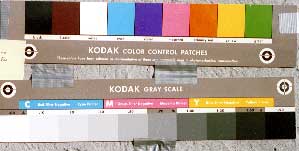 |
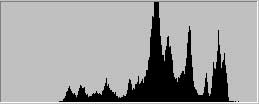 fig. 1 fig. 1 |
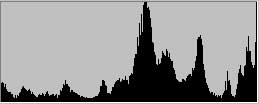 fig. 2 fig. 2 |
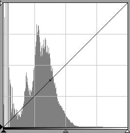
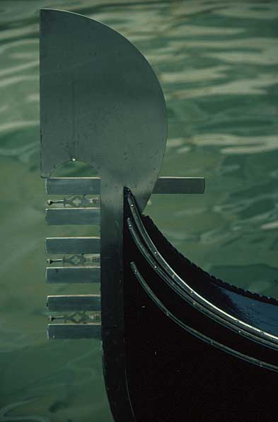
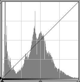
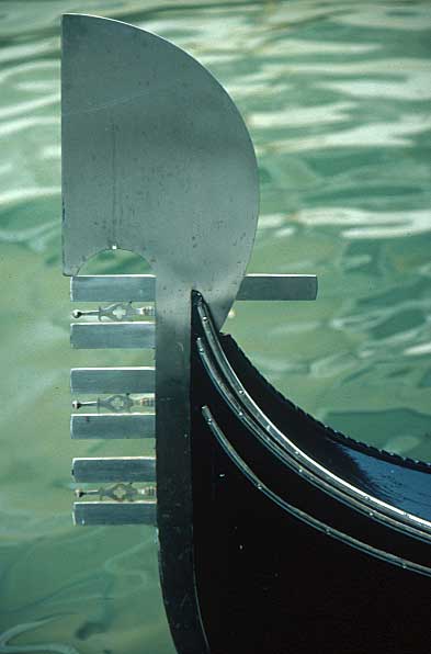
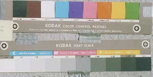
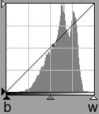
| Failure to specify the black/white points
causes
the computer to display black and white improperly (fig. 1). An
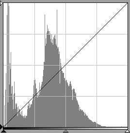
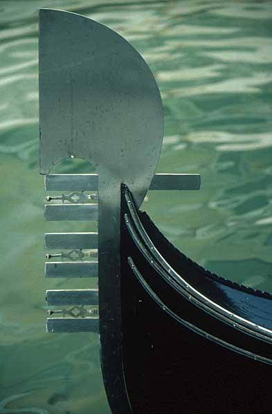
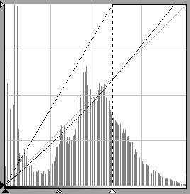
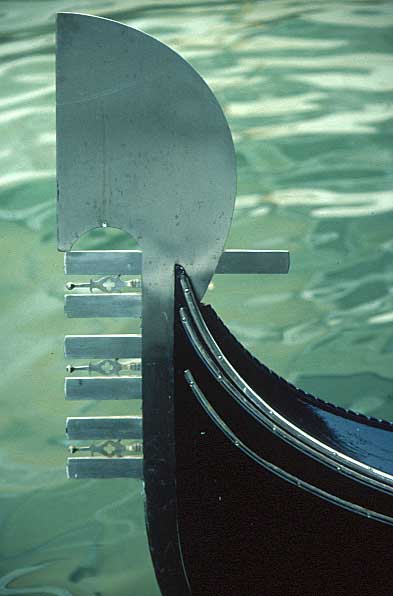
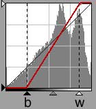
image with the black/white points properly set will have a histogram that
spans the full range of tones (fig. 2). |
In this example, the initial scanner histogram has gaps between the margins of the graph
and the left-most and right-most portions the histogram so that the darkest tone
in the image is not black and the lightest is not white.
 Input
histogram
Input
histogram
Setting the black and white points may be accomplished in several ways. The most direct way is
move the black pointer (b) until it is immediately below the left edge of the
histogram and the white pointer (w) until it is immediately below the right edge
of the histogram. Using the black eye dropper to sample an identifiably black
tone and the white eye dropper to sample an identifiably white tone have exactly
the same effect. Another method is to press the 'auto' or the 'cont' buttons
and let the computer do it. NikonScan, however, doesn't merely place the
pointers at the extreme edges of the histogram. For the black point it moves the
pointer to the right beyond the left edge until the darkest 0.3% of the pixels
become black. For the white point it moves the pointer to the left beyond the
right edge until the brightest 0.3% of the pixels become white. (You may redefine
the black and white point settings in the 'misc' color tab in the
preferences. Note that Photoshop sets its clipping point at 0.5% at both
ends.) The
reasoning behind this is that NikonScan assumes the extreme 0.3% of the pixels are unrepresentative
of the image (e.g. noise) and can be thrown into the extreme values; they are
'clipped'. In addition, the way in which the auto b/w point is set changed with
NikonScan 2.5. Instead of operating on the RGB tone curve (going top-down), NikonScan
individually sets the b/w points on the underlying red, green, and blue curves
(going bottom-up).
Theoretically this achieves the greatest tonal separation. If the b/w
pointer settings among the red, green, and blue curves differ greatly, however, it means that the individual
color channels have undergone radically different contrast adjustments. It may be
difficult to restore the color balance using only curves. The balance may be
achieved by adjusting the analog gain of the underlying color channels until the
relative positions of the b/w pointers among them are restored.
 Curve with b/w point setting
and output histogram
Curve with b/w point setting
and output histogram
When you set the b/w points you're really making 2 curve adjustments:
the left-end of the histogram is shifted down to zero, and the right-end is
shifted up to 255. The net effect is a contrast change curve applied to the
histogram. The equivalent tone curve method to setting the b/w point is
demonstrated in fig. 1.
Note that the curve (in red) has an "S" shape characteristic of an
increase in contrast.
Setting the Black-White Points in
Hardware
In contrast to the previous software method using curves, setting the
black-white point in hardware works in reverse by modifying the shape of the
histogram until it fits within the graph's margins. On the Nikon LS, for
example, this means using analog gain, which controls the luminance of the
scanner LEDs. Increasing analog gain is similar to increasing the exposure
in an enlarger so that more light passes through the denser areas of the image.
Usually this method is used in conjunction with transparency films, which are
more likely to have dense tonal areas. The reason for using this method is
that by forcing the image to span the scanner's density range in the analog
domain samples are obtained potentially for all 256 values, assuring a
continuously toned image.
Here is an example using this method done with a Kodachrome image: